Model Fit Diagnostics with the Q Statistic • fungwas

Overview

In this vignette we show how to use the Q statistic in fungwas to compare parametric mappings of quantile GWAS slopes to competing distributional models.

The Q statistic is defined as

[ Q = (b - W ){-1} (b - W ),]

where:

1. are the observed quantile slopes,
(W ) are the slopes implied by the fitted parametric model,
() is the estimated covariance of the slopes.

A small Q indicates that the model is consistent with the observed slopes. A larger Q indicates misfit.

Important caveat: Because the covariance estimates () used here are approximate (especially under diagonal or plugin modes), the Q statistic should be interpreted heuristically. It is not a formal likelihood-ratio test. In practice, the main diagnostic is whether a model’s average Q is much smaller than that of an alternative model. Absolute calibration against chi-square reference distributions is unreliable.

Example: vQTL vs Log-normal Model

We simulate phenotypes from a mean + variance QTL model, and then compare fit against a log-normal model where the SNP only influences the mean (with variance tied through the log-normal link).

# -------------------------
# 1. Simulate genotypes
# -------------------------
N <- 15000
P <- 500
maf <- runif(P, 0.05, 0.5)
G <- matrix(rbinom(N * P, 2, rep(maf, each = N)), nrow = N, ncol = P)
colnames(G) <- paste0("SNP", seq_len(P))

# -------------------------
# 2. Define true effects
# -------------------------
beta_mu_true     <- rnorm(P) / 40
beta_sigma2_true <- rnorm(P) / 40

# -------------------------
# 3. Simulate phenotype
# -------------------------
mu0 <- 4.0
sd0 <- 0.6

mu <- mu0 + G %*% beta_mu_true
sigma2 <- sd0^2 + G %*% beta_sigma2_true
sigma2[sigma2 <= 0] <- 1e-4  # guard against negative variances

Y <- rnorm(N, mean = mu, sd = sqrt(sigma2))

Stage 1: Quantile GWAS

We first compute quantile slopes using RIF regression.

taus <- seq(0.05, 0.95, 0.05)
stage1 <- quantile_gwas(
  Y, G,
  taus = taus,
  benchmark = FALSE,
  verbose = FALSE
)

Stage 2: Correct Model (Mean + Variance QTL)

We map slopes to mean and variance parameters using make_weights_vqtl.

W_var <- make_weights_vqtl(taus, stage1$q_tau, mu = mean(Y), sd = sd(Y))

fit_correct <- param_gwas(
  stage1,
  transform = "custom_W",
  transform_args = list(W = W_var),
  se_mode = "dwls"
)

Stage 2: Wrong Model (Log-normal)

We now compare against a log-normal distribution. Here, effects on the meanlog implicitly alter both the mean and variance, but without an independent variance parameter.

logY <- log(Y)
fitlog <- list(
  estimate = c(meanlog = mean(logY), sdlog = sd(logY))
)
q_tau <- as.numeric(quantile(Y, taus, type = 8))

dist_cdf <- function(y, params) plnorm(y, meanlog = params$meanlog, sdlog = params$sdlog)
dist_pdf <- function(y, params) dlnorm(y, meanlog = params$meanlog, sdlog = params$sdlog)

grad_fd_meanlog <- make_fd_grad("meanlog", dist_cdf)
grad_fd_sdlog   <- make_fd_grad("sdlog", dist_cdf)

W_fd <- make_weights_generic(
  taus, q_tau, dist_cdf, dist_pdf,
  params = list(meanlog = fitlog$estimate[1], sdlog = fitlog$estimate[2]),
  grad_funcs = list(beta_meanlog = grad_fd_meanlog,
                    beta_sdlog   = grad_fd_sdlog)
)

fit_wrong <- param_gwas(
  stage1,
  transform = "custom_W",
  transform_args = list(W = W_fd),
  se_mode = "dwls"
)

Compare Q Statistics

cat("\n--- Model Comparison ---\n")
#> 
#> --- Model Comparison ---
cat("Correct model Q (per SNP):\n")
#> Correct model Q (per SNP):
print(summary(fit_correct$Q))
#>    Min. 1st Qu.  Median    Mean 3rd Qu.    Max. 
#>   0.595   3.433   4.992   5.747   7.322  19.607

cat("\nWrong model Q (per SNP):\n")
#> 
#> Wrong model Q (per SNP):
print(summary(fit_wrong$Q))
#>    Min. 1st Qu.  Median    Mean 3rd Qu.    Max. 
#>  0.6344  3.5250  5.0815  5.8670  7.2588 21.6910

cat("\nAverage Q difference (wrong - correct):\n")
#> 
#> Average Q difference (wrong - correct):
mean(fit_wrong$Q - fit_correct$Q)
#> [1] 0.1196326

plot(fit_correct$Q - fit_wrong$Q,
     main = "Q(correct) - Q(wrong) per SNP",
     ylab = "ΔQ", xlab = "SNP index")
abline(h = 0, col = "red")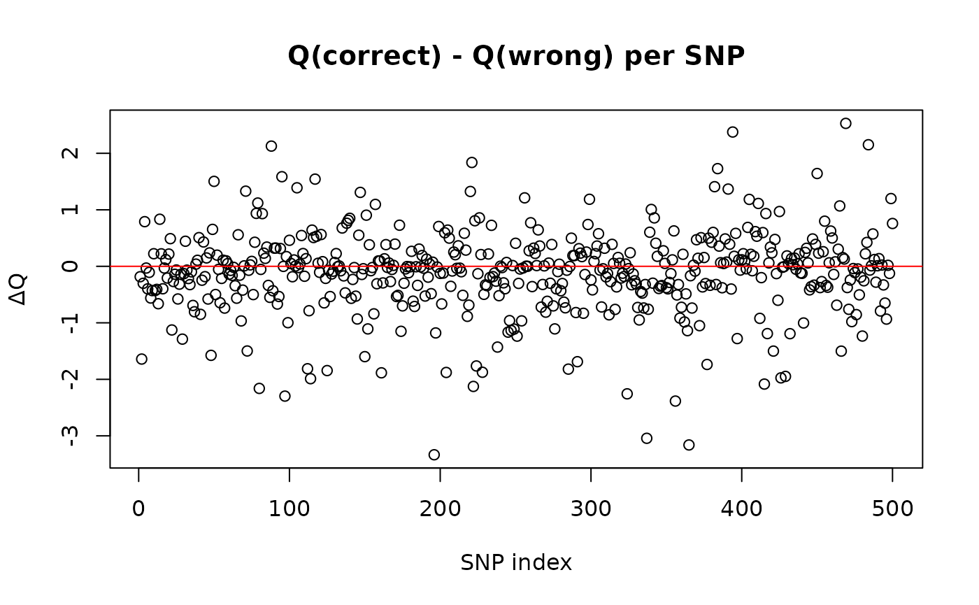

In this example, the true vQTL model yields systematically lower Q values than the misspecified log-normal model, confirming that the variance effects are necessary to explain the quantile slopes.

Key Takeaways

The Q statistic in fungwas is a heuristic measure of model adequacy, not a calibrated chi-square test.
When comparing competing models, a large difference in average Q provides evidence for which model better captures the distributional shape of the phenotype.
However, because SEs are approximate, absolute reference to chi-square distributions is discouraged.
In practice, Q is best used to ask: Does my chosen parametric system capture the quantile slopes better than a simpler alternative?

Conclusion

The Q statistic provides a useful way to compare alternative parametric models in fungwas. It should be seen as a diagnostic tool, helping identify whether variance effects, mixtures, or other parameters are needed to describe the phenotype distribution, rather than as a formal hypothesis test.