3  Evaluating DNA Language Models

Abstract

In this chapter, we’ll discuss how we can evaluate whether our DNA language model has learned anything. We pick a simple, biologically informed evaluation. We compare the plausibility (according to the model) of 2 classes of mutations: missense mutations which change a protein and synonymous mutations which do not change the protein. To do this, we’ll take a gene (DRD2) and introduce synthetic mutations that are either missense or synonymous.

All scripts for this chapter are found here: https://github.com/MichelNivard/Biological-language-models/tree/main/scripts/DNA/Chapter_3

3.1 Introduction

In Chapters 1 and 2, we introduced the process of preparing DNA sequences and training a BERT language model for genomic data. In this chapter, we will turn our attention to how single nucleotide mutations can be systematically generated and evaluated using the trained DNA language model.

These synthetic mutations can form the basis for an evaluation of our DNA language model.

This chapter has two goals:

• To explain to machine learning readers how to enumerate synonymous and missense mutations based on the standard genetic code, and why this is biologically meaningful. Consider the Khan Academy “AP Bio” course if this chapter doesn’t really offer enough for you https://www.khanacademy.org/science/ap-biology

• To explain to bioinformatics and genetics readers how the Masked Language Modeling (MLM) objective provides a way to compute the pseudo-log-likelihood (PLL) of entire sequences and to score mutations in terms of their “naturalness” under the trained model.

3.2 Biological Background: The Genetic Code and Mutation Types

Before diving into code, it’s useful to recall the basics of how DNA encodes proteins. DNA is transcribed into RNA, and RNA is translated into proteins using codons, groups of three nucleotides. Each codon corresponds to a specific amino acid, this mapping is called the genetic code.

Figure 3.1 DNA is transcribed to RNA then translated to amino acids which form proteins. Source: https://www.khanacademy.org/science/ap-biology/gene-expression-and-regulation/translation/a/intro-to-gene-expression-central-dogma

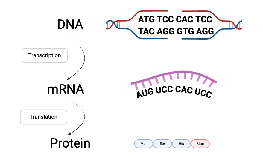
Crucially, some amino acids can be encoded by multiple codons, a property called degeneracy. This degeneracy is why synonymous mutations exist — changes in the DNA sequence that do not alter the resulting amino acid. In contrast, missense mutations alter the encoded amino acid, which may change protein function.

This distinction between synonymous and missense mutations will allow us to systematically categorize the impact of each possible single nucleotide substitution. Below is the standard genetic code table; it contains a full translation from DNA to protein.

Codon	Amino Acid	Codon	Amino Acid	Codon	Amino Acid	Codon	Amino Acid
TTT	F	TTC	F	TTA	L	TTG	L
TCT	S	TCC	S	TCA	S	TCG	S
TAT	Y	TAC	Y	TAA	Stop	TAG	Stop
TGT	C	TGC	C	TGA	Stop	TGG	W
CTT	L	CTC	L	CTA	L	CTG	L
CCT	P	CCC	P	CCA	P	CCG	P
CAT	H	CAC	H	CAA	Q	CAG	Q
CGT	R	CGC	R	CGA	R	CGG	R
ATT	I	ATC	I	ATA	I	ATG	M
ACT	T	ACC	T	ACA	T	ACG	T
AAT	N	AAC	N	AAA	K	AAG	K
AGT	S	AGC	S	AGA	R	AGG	R
GTT	V	GTC	V	GTA	V	GTG	V
GCT	A	GCC	A	GCA	A	GCG	A
GAT	D	GAC	D	GAA	E	GAG	E
GGT	G	GGC	G	GGA	G	GGG	G

A single nucleotide mutation can cause:

• A synonymous mutation: The amino acid does not change, meaning the mutation is “silent” in terms of protein sequence. For example, in row 1 of the table, we see that if we mutate the codon TTT to TTC, both before and after the mutation the amino acid F (phe) is produced. While it’s not guaranteed by any means that a synonymous mutation is entirely harmless, they’re very likely to be harmless.
• A missense mutation: The amino acid changes, potentially altering protein structure and function. For example, in row 1 of the table, we see that if we mutate the codon TTT to TTA, the amino acid F (phe) is replaced by L (leu) in the protein, potentially changing the function. While missense mutations aren’t always damaging, they are far more likely to be damaging.

Earlier, we trained a DNA language model on coding sequences for humans, and I actually expanded that to a training run of 2 epochs (the data was all used twice) on 500k sequences from 13 vertebrate species. This model should, with probabilities slightly above chance,

3.3 Creating All Single-Nucleotide Mutants

The code in this section systematically generates every possible single nucleotide substitution across the input sequence. Since each codon consists of three nucleotide’s, and each nucleotide can mutate into three alternatives, there are up to 9 potential codon variants for each original codon.

Tip

The data generated by applying this “mutator” to the DRD2 (Dopamine receptor D2) gene is on Hugging Face: https://huggingface.co/datasets/MichelNivard/DRD2-mutations

For each mutation, we check the original amino acid and the new amino acid using the standard genetic code table. This allows us to classify each mutation as either:

• Synonymous: Same amino acid, no apparent change to the protein.

• Missense: Different amino acid, potential change to protein function.

This step is crucial in genomics, where we often want to prioritize functional variants — mutations that actually change protein products, rather than silent changes that do not.

I have a preference for R myself, so I wrote this specific job in R. We provide the gene sequence, starting at the start codon; I use the dopamine receptor gene DRD2. Based on the genetic code, which translates DNA to the amino acids that eventually are produced, we then write code to mutate each codon in a gene.

FOr the demo we’ll manually imput the gene:

DRD2 <- "ATGGATCCACTGAATCTGTCCTGGTATGATGATGATCTGGAGAGGCAGAACTGGAGCCGGCCCTTCAACGGGTCAGACGGGAAGGCGGACAGACCCCACTACAACTACTATGCCACACTGCTCACCCTGCTCATCGCTGTCATCGTCTTCGGCAACGTGCTGGTGTGCATGGCTGTGTCCCGCGAGAAGGCGCTGCAGACCACCACCAACTACCTGATCGTCAGCCTCGCAGTGGCCGACCTCCTCGTCGCCACACTGGTCATGCCCTGGGTTGTCTACCTGGAGGTGGTAGGTGAGTGGAAATTCAGCAGGATTCACTGTGACATCTTCGTCACTCTGGACGTCATGATGTGCACGGCGAGCATCCTGAACTTGTGTGCCATCAGCATCGACAGGTACACAGCTGTGGCCATGCCCATGCTGTACAATACGCGCTACAGCTCCAAGCGCCGGGTCACCGTCATGATCTCCATCGTCTGGGTCCTGTCCTTCACCATCTCCTGCCCACTCCTCTTCGGACTCAATAACGCAGACCAGAACGAGTGCATCATTGCCAACCCGGCCTTCGTGGTCTACTCCTCCATCGTCTCCTTCTACGTGCCCTTCATTGTCACCCTGCTGGTCTACATCAAGATCTACATTGTCCTCCGCAGACGCCGCAAGCGAGTCAACACCAAACGCAGCAGCCGAGCTTTCAGGGCCCACCTGAGGGCTCCACTAAAGGAGGCTGCCCGGCGAGCCCAGGAGCTGGAGATGGAGATGCTCTCCAGCACCAGCCCACCCGAGAGGACCCGGTACAGCCCCATCCCACCCAGCCACCACCAGCTGACTCTCCCCGACCCGTCCCACCATGGTCTCCACAGCACTCCCGACAGCCCCGCCAAACCAGAGAAGAATGGGCATGCCAAAGACCACCCCAAGATTGCCAAGATCTTTGAGATCCAGACCATGCCCAATGGCAAAACCCGGACCTCCCTCAAGACCATGAGCCGTAGGAAGCTCTCCCAGCAGAAGGAGAAGAAAGCCACTCAGATGCTCGCCATTGTTCTCGGCGTGTTCATCATCTGCTGGCTGCCCTTCTTCATCACACACATCCTGAACATACACTGTGACTGCAACATCCCGCCTGTCCTGTACAGCGCCTTCACGTGGCTGGGCTATGTCAACAGCGCCGTGAACCCCATCATCTACACCACCTTCAACATTGAGTTCCGCAAGGCCTTCCTGAAGATCCTCCACTGCTGA"
nchar(DRD2)/3

Thewn we’ll need to encode the genertic code, to translate between nucleotides and amino-acids:

# Genetic code table (Standard Code)
genetic_code <- c(
  "TTT"="F", "TTC"="F", "TTA"="L", "TTG"="L",
  "TCT"="S", "TCC"="S", "TCA"="S", "TCG"="S",
  "TAT"="Y", "TAC"="Y", "TAA"="Stop", "TAG"="Stop",
  "TGT"="C", "TGC"="C", "TGA"="Stop", "TGG"="W",
  "CTT"="L", "CTC"="L", "CTA"="L", "CTG"="L",
  "CCT"="P", "CCC"="P", "CCA"="P", "CCG"="P",
  "CAT"="H", "CAC"="H", "CAA"="Q", "CAG"="Q",
  "CGT"="R", "CGC"="R", "CGA"="R", "CGG"="R",
  "ATT"="I", "ATC"="I", "ATA"="I", "ATG"="M",
  "ACT"="T", "ACC"="T", "ACA"="T", "ACG"="T",
  "AAT"="N", "AAC"="N", "AAA"="K", "AAG"="K",
  "AGT"="S", "AGC"="S", "AGA"="R", "AGG"="R",
  "GTT"="V", "GTC"="V", "GTA"="V", "GTG"="V",
  "GCT"="A", "GCC"="A", "GCA"="A", "GCG"="A",
  "GAT"="D", "GAC"="D", "GAA"="E", "GAG"="E",
  "GGT"="G", "GGC"="G", "GGA"="G", "GGG"="G"
)

Then we define a function, which for a codon, in a gene, applied all mutations (e.g. each of the 3 based is mutated to G,C,T and A). It stores a whole bunch of info on the mutation, essential is that it also encodes whether the mutation is synonymous, or missense, but also which amino-acid is changed to which other amino-acid. This could allow you to later go back

# Function to get all mutations for a codon
mutate_codon <- function(codon, codon_index, full_sequence) {
  nucleotides <- c("A", "T", "C", "G")
  mutations <- data.frame()
  
  original_aa <- genetic_code[[codon]]
  
  for (pos in 1:3) {
      original_base <- substr(codon, pos, pos)
      for (nuc in nucleotides) {
          if (nuc != original_base) {
              # Mutate the codon at this position
              mutated_codon <- codon
              substr(mutated_codon, pos, pos) <- nuc
              mutated_aa <- genetic_code[[mutated_codon]]
              
              # Create the mutated sequence
              mutated_sequence <- full_sequence
              start <- (codon_index - 1) * 3 + 1
              substr(mutated_sequence, start, start+2) <- mutated_codon
              
              mutation_type <- if (mutated_aa == original_aa) "synonymous" else "missense"
              
              mutations <- rbind(mutations, data.frame(
                  codon_index = codon_index,
                  position = pos,
                  original_codon = codon,
                  mutated_codon = mutated_codon,
                  original_aa = original_aa,
                  mutated_aa = mutated_aa,
                  mutation_position = (codon_index -1)*3 + pos,
                  mutation_type = mutation_type,
                  sequence = mutated_sequence
              ))
          }
      }
  }
  return(mutations)
}

Then we define the main function, which applies the mutations to the whole sequence, storing all possible single base mutations:

# Main function to process the whole sequence
mutate_sequence <- function(dna_sequence) {
  codons <- strsplit(dna_sequence, "")[[1]]
  codons <- sapply(seq(1, length(codons), by=3), function(i) paste(codons[i:(i+2)], collapse=""))
  all_mutations <- data.frame()
  
  for (i in seq_along(codons)) {
      codon <- codons[i]
      mutations <- mutate_codon(codon, i, dna_sequence)
      all_mutations <- rbind(all_mutations, mutations)
  }
  return(all_mutations)
}

We apply these functionsto the DRD2 sequence, and we store all mutated sequences and a bunch of meta data.

# Example usage
sequence <- DRD2
mutations <- mutate_sequence(sequence)

# Filter synonymous and missense if needed
synonymous_mutations <- subset(mutations, mutation_type == "synonymous")
missense_mutations <- subset(mutations, mutation_type == "missense")

source <- c(NA,"wildtype",DRD2)

output <- rbind(source,mutations[,7:9])

write.csv(file="DRD2_mutations.csv",output)

3.4 Evaluating base position likelihoods with a BERT Model

In machine learning terms, the MLM loss is the negative log likelihood (NLL) of the correct nucleotide. For example, if the correct nucleotide is “A” at a given position, and the model assigns “A” a probability of 0.8, then the contribution to the loss is:

\[loss = −ln(0.8) = 0.22\]

The lower this value, the better the model’s confidence matches reality — indicating that the nucleotide was expected. Near the end of training our models loss hovered around 1.09, meaning that the average true base had a predicted probability of ±34%. The loss is highly dependent on the tokenizer, for example if we would have used a more complex tokenizer with say 100 options for each next token (encoding for example all 3-mer combinations of bases: A,C,T,G,AA,AC,AT,AG etc etc until GGA,GGG) the the probability of geting the one correct token is way lower as the base rate is way lower!

When we compute the pseudo-log-likelihood (PLL) for an entire sequence, we mask and score each position, adding up these log probabilities:

\[log⁡P(nucleotide_1)+log⁡P(nucleotide_2)+ ⋯ +log⁡P(nucleotide_n)​\]

This sum is the total log likelihood of the sequence under the model — it quantifies how natural the model thinks the sequence is.

First we load the model I trained in Chapter 2, if you trained your own on more data, or for longer, or want to evaluate a different model you can load those yourself easily.

from transformers import AutoTokenizer, AutoModelForMaskedLM
import torch
import pandas as pd

# Load model & tokenizer
model_name = "MichelNivard/DNABert-CDS-13Species-v0.1"  # Replace if needed
tokenizer = AutoTokenizer.from_pretrained(model_name)
model = AutoModelForMaskedLM.from_pretrained(model_name)
model.eval()

device = torch.device("cuda" if torch.cuda.is_available() else "cpu")
model.to(device)

# Maximum context length — BERT's trained context window
MAX_CONTEXT_LENGTH = 512

3.4.1 Estimating the effects of all mutations

Then we define two functions (we’re back to python here) to compute: 1) the pseudo-likelihood of the whole sequence up to 512 bases, as that is the sequence length we trained DNABert for (in full-scale applications, you’d use a longer sequence length), and 2) the log-likelihood ratio of the mutation vs. the wildtype (original DRD2 sequence).

def compute_log_likelihood(sequence, tokenizer, model):
    """Compute pseudo-log-likelihood (PLL) for the first 512 bases."""
    tokens = tokenizer(sequence, return_tensors='pt', add_special_tokens=True)
    input_ids = tokens['input_ids'].to(device)
    attention_mask = tokens['attention_mask'].to(device)

    log_likelihood = 0.0
    seq_len = input_ids.shape[1] - 2  # Exclude [CLS] and [SEP]

    with torch.no_grad():
        for i in range(1, seq_len + 1):
            masked_input = input_ids.clone()
            masked_input[0, i] = tokenizer.mask_token_id

            outputs = model(masked_input, attention_mask=attention_mask)
            logits = outputs.logits

            true_token_id = input_ids[0, i]
            log_probs = torch.log_softmax(logits[0, i], dim=-1)
            log_likelihood += log_probs[true_token_id].item()

    return log_likelihood


def compute_mutant_log_likelihood_ratio(wild_type, mutant, position, tokenizer, model):
    """Compare wild type and mutant likelihood at a single position (within 512 bases)."""
    assert len(wild_type) == len(mutant), "Wild type and mutant must have the same length"
    assert wild_type[position] != mutant[position], f"No mutation detected at position {position + 1}"

    tokens = tokenizer(wild_type[:MAX_CONTEXT_LENGTH], return_tensors='pt', add_special_tokens=True)
    input_ids = tokens['input_ids'].to(device)
    attention_mask = tokens['attention_mask'].to(device)

    mask_position = position + 1  # Shift for [CLS] token

    masked_input = input_ids.clone()
    masked_input[0, mask_position] = tokenizer.mask_token_id

    with torch.no_grad():
        outputs = model(masked_input, attention_mask=attention_mask)
        logits = outputs.logits

        log_probs = torch.log_softmax(logits[0, mask_position], dim=-1)

    wild_base_id = tokenizer.convert_tokens_to_ids(wild_type[position])
    mutant_base_id = tokenizer.convert_tokens_to_ids(mutant[position])

    log_prob_wild = log_probs[wild_base_id].item()
    log_prob_mutant = log_probs[mutant_base_id].item()

    return log_prob_wild - log_prob_mutant

3.4.2 The Likelihood Ratio to evaluate mutations

The log-likelihood ratio (LLR) compares how much more (or less) likely the wild-type sequence is compared to a mutant sequence, given the DNA language model. Specifically, we compare the log-likelihood of the correct wild-type nucleotide to the log likelihood of the mutant nucleotide at the mutated position only.

\[LLR = log ⁡ P ( wild-type nucleotide ∣ context ) − log ⁡ P ( mutant nucleotide ∣ context )\]

This metric is widely used in bioinformatics because it focuses on the exact site of the mutation, instead of comparing entire sequences. A positive LLR indicates the wild-type is favored by the model (the mutation is unlikely and therefore possibly deleterious), while a negative LLR means the mutant is more likely (the mutation is neutral or maybe even protective).

We then apply these functions to all the synthetic DRD2 mutations we generated (in the first 512 bases) to evaluate whether the DNABert we trained thinks the missense mutations are generally less likely, and therefore possibly damaging, given the model.

# Load dataset directly from Hugging Face dataset repo
dataset_url = "https://huggingface.co/datasets/MichelNivard/DRD2-mutations/raw/main/DRD2_mutations.csv"
df = pd.read_csv(dataset_url)

# Find wild-type sequence
wild_type_row = df[df['mutation_type'] == 'wildtype'].iloc[0]
wild_type_sequence = wild_type_row['sequence'][:MAX_CONTEXT_LENGTH]

results = []

# Process all sequences
for idx, row in df.iterrows():
    sequence = row['sequence'][:MAX_CONTEXT_LENGTH]
    mutation_type = row['mutation_type']
    mutation_position = row['mutation_position'] - 1  # Convert 1-based to 0-based

    # Skip mutants where the mutation position is beyond 512 bases
    if mutation_type != 'wildtype' and mutation_position >= MAX_CONTEXT_LENGTH:
        continue

    print(idx)

    llr = None
    log_prob_wild = None
    prob_wild = None

    if mutation_type != 'wildtype':
        llr, log_prob_wild, prob_wild = compute_mutant_log_likelihood_ratio(
            wild_type_sequence, sequence, int(mutation_position), tokenizer, model
        )

    # append results for each mutation:
    results.append({
        'sequence': sequence,
        'mutation_type': mutation_type,
        'pll': 0,
        'llr': llr,
        'wildtype_log_prob': log_prob_wild,
        'wildtype_prob': prob_wild,
        'mutation_position': mutation_position + 1
    })


# Convert to DataFrame for saving or inspection
results_df = pd.DataFrame(results)

# Save or print results
print(results_df)

# Optionally, save to CSV
results_df.to_csv("sequence_log_likelihoods.csv", index=False)

3.4.3 Language Models Provide Biological Insight through the likelihood ratio

Why do we care about these log likelihoods and log likelihood ratios? Because they provide a direct, data-driven estimate of how plausible or “natural” each mutated sequence looks to the model compared to the wild type sequence. Since the model was trained on real DNA sequences, sequences with high likelihoods resemble biological reality, while sequences with low likelihoods deviate from patterns the model has learned. A high “mutation log likelihood ratio” corresponds to the model strongly favoring the reference sequences over the mutation(Meier et al. 2021). This test lets us flag potentially deleterious mutations (those with sharp likelihood drops), prioritize candidate variants for functional follow-up, or even explore adaptive evolution by identifying mutations that DNA BERT “likes” more than the wild-type

To explore our result here, we can plot the LLR versus the position within the DRD2 gene, this can give us insight into the location within the coding sequence where we find unlikely (and therefore potentially damaging) mutations. in the plot below a LOW LLR means the variant is unlikely. Most variants cluster around a neutral LLR, consistent with some statistical noise.

import numpy as np
import pandas as pd
import matplotlib.pyplot as plt
import seaborn as sns

# Filter to only mutations (skip wildtype which has no llr)
plot_df = results_df[results_df['mutation_type'].isin(['synonymous', 'missense'])].copy()


# Optional: Clip LLR to avoid excessive sizes
plot_df['size'] = plot_df['llr'].clip(-5, 5)  # LLRs smaller than -5 get maximum size

# Scatter plot with enhanced size scaling
plt.figure(figsize=(14, 5))
sns.scatterplot(
    x='mutation_position', 
    y='llr', 
    hue='mutation_type', 
    size='size',  # Use clipped size column
    sizes=(20, 200),  # Bigger range for better visibility
    alpha=0.7, 
    palette={'synonymous': 'green', 'missense': 'orange'},
    data=plot_df
)
plt.axhline(0, color='gray', linestyle='--', label='Neutral LLR')
plt.title('Mutation Log Likelihood Ratio (LLR) Along DRD2 Gene')
plt.xlabel('Position in Gene')
plt.ylabel('Log Likelihood Ratio (LLR)')
plt.legend(title='Mutation Type', bbox_to_anchor=(1.02, 1), loc='upper left')
plt.grid(True, linestyle='--', alpha=0.5)
plt.show()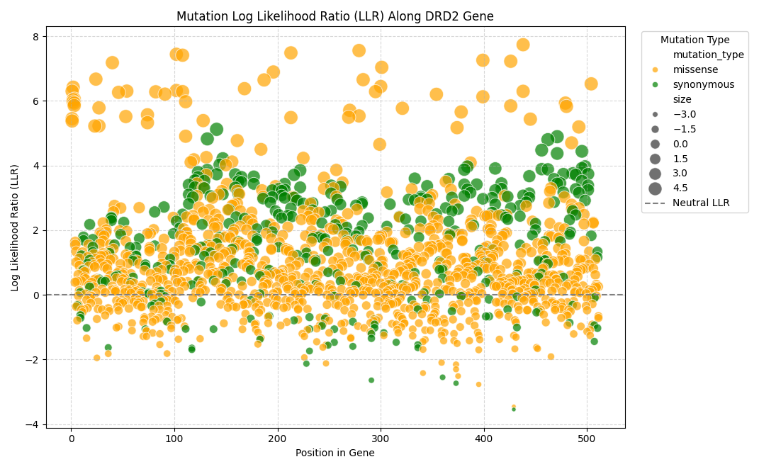

Figure 3.2 The LLR for the mutation (y-axis) give the position in the DRD2 gene (x-axis). High values indicate the reference, or wild, type sequence is far more likely than the mutation. Very high LLR values are almost exclusively missense mutations, consistent with a DNA model able to pick up deleterious variants based on its training

It’s obvious from Figure 3.2 that 1. really almost all very unlikely mutations (positive LLR) are missense mutations and 2. There are potentially certain locations within this particular coding sequence where there is an abundance of unlikely mutations packed closely together, these could be regions that are intolerant to deleterious mutations.

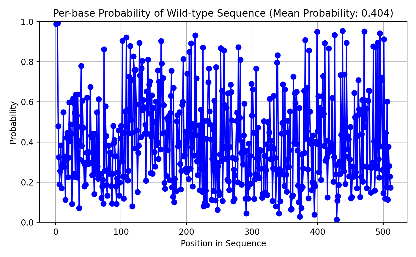
It’s important to not get overconfident in our predictions! Remember this is a relatively tiny DNA sequence model (±5m parameters) we trained on sequences for 13 fairly randomly picked vertebrate species. Let’s look at the likelihood of the true base in the references (wild-type) sequence given the model. The mean probability is 40% (Figure 3.3), given the model essentially is trying to pick between 4 tokens (G,C,T & A) 40% is considerably better than chance! It’s also clear the probability is not even across the gene, the first few bases are almost certain (almost all coding sequences in these species start with the start codon ATG, the model obviously learned this). After that, there is quite a spread, which is logical I think, in many places across the sequence the specific base might be very obvious, as all three alternates might be missense mutations, but in other spots one, two or even all three alternate tokens might be synonymous, and perhaps even present in the analog gene in the other 12 species we trained our model on! This would make the model FAR less certain about the true base at that location.

Figure 3.3 The probability of the base in the reference, or wild type, sequence given the DNABert model we trained. The model clearly performed above random (random guessing would be 1 in 4, or 25%).

3.5 Self-Study Exercises

You have reached a key point where you now are a “consumer” of DNA language models. If you have followed along you should be able to run them on a sequence of our choosing. But to become a savvy or discerning consumer (let that cabernet breath, roll it around the glass…) of DNA language models, you’ll have to evaluate them on a benchmark that matches your application. The exercises below are meant to give you a taste of evaluating a few models. The hard exercises also set us up for the next few chapters by pulling in external evolutionary salient data. There are people who think long and hard about model evaluation (Patel et al. 2024; Tang et al. 2024) and if you are to do rigorous evaluation for an academic project/paper it’ll pay off to catch up on the literature.

Tip

If you want a good Masters/PhD term project with limited compute demands, or optimal self-study try some of the following excersizes:

1. (easy) Evaluate about 100 genes split the variants into synonymous, missense, start-lost (the start coding is changed by the mutation), stop-gained (a specific amino-acid is mutated to a stop coding) and reproduce those 4 rows in (Benegas, Batra, and Song 2023) figure 4. Think critically whether you want to consider alternate metrics for “fit” we used LLR in this chapter, but others used cosine distance, or dot-product between wild-type and mutated sequence embedding as a measure of deleteriousness. Do the other metrics more clearly separate stop-gained from missense from synonymous?

2. (medium) Evaluate about 100 genes split the synthetic variants into synonymous, missense, start-lost, stop-gained and reproduce those 4 rows in (Benegas, Batra, and Song 2023) figure 4. Do so for 3 DNA language models, the one we trained in Chapter 2 (use your own, or if you didn’t train one the one I made available: https://huggingface.co/MichelNivard/DNABert-CDS-13Species-v0.1 ) a medium sized (500m parameters) nucleotide transformer (Dalla-Torre et al. 2024) (https://huggingface.co/InstaDeepAI/nucleotide-transformer-v2-500m-multi-species) and DNABERT-2 (Zhou et al. 2023) (https://huggingface.co/zhihan1996/DNABERT-2-117M).

3. (hard) Evaluate about 100 genes split the synthetic variants into synonymous, missense, start-lost , stop-gained and reproduce those 4 rows in (Benegas, Batra, and Song 2023) figure 4. Do so for 3 DNA language models, the one we trained in Chapter2 ( use your own, or if you didn’t train one the one I made available: https://huggingface.co/MichelNivard/DNABert-CDS-13Species-v0.1 ) a medium sized (500m parameters) nucleotide transformer (Dalla-Torre et al. 2024) (https://huggingface.co/InstaDeepAI/nucleotide-transformer-v2-500m-multi-species) and DNABERT-2 (Zhou et al. 2023) (https://huggingface.co/zhihan1996/DNABERT-2-117M). Allign the DNA sequences with at least one external track form the UCSC genome browser, for example the allele frequencies in 1000 genomes, or the 100 way alignment across species (https://hgdownload.soe.ucsc.edu/goldenPath/hg38/multiz100way/). Establish whether mutations to bases that are rarely variant(MAF < 5%), or variants that are never observed (freq = 0%), or those to bases that are less conserved are less likely according to the model.

3.6 Further reading

• A paper diving deeper into the the nature of proteins for which the likelihood ratio is able to detect the deleteriousness of mutations. It turns out the LLR is most informative for proteins with a certain perplexity given the model, which puts boundaries on the set of proteins for which the LLR is useful.

• A blog post implementing the LLR, and other scoring metrics form a recent paper(Meier et al. 2021), for protein language models (specifically ESM2).

3.7 Summary

This chapter introduced key pieces that are essential for those who want to train, or just understand, DNA Language models.

• We explored how to systematically generate all synonymous and missense mutations in a gene, these simulated mutations then form an important part in initial evaluation of our model.
• We discussed how to compute the log-likelihood of sequences, and log-likelihood ratio of a single mutation using DNA BERT. These metrics are a proxy for how natural the model considers each sequence.
• We finally used these simulated mutations and some knowledge of biology (whether the mutations are synonymous or missense) to validate that our language model actually did do some learning.
• We reviewed possible exercises that could help you become a better consumer of genomic language models by critically evaluating them.

The analyses outlined in this chapter form the foundation for variant effect prediction using genomic language models.

Benegas, Gonzalo, Sanjit Singh Batra, and Yun S. Song. 2023. “DNA Language Models Are Powerful Predictors of Genome-Wide Variant Effects.” Proceedings of the National Academy of Sciences 120 (44). https://doi.org/10.1073/pnas.2311219120.

Dalla-Torre, Hugo, Liam Gonzalez, Javier Mendoza-Revilla, Nicolas Lopez Carranza, Adam Henryk Grzywaczewski, Francesco Oteri, Christian Dallago, et al. 2024. “Nucleotide Transformer: Building and Evaluating Robust Foundation Models for Human Genomics.” Nature Methods 22 (2): 287–97. https://doi.org/10.1038/s41592-024-02523-z.

Meier, Joshua, Roshan Rao, Robert Verkuil, Jason Liu, Tom Sercu, and Alexander Rives. 2021. “Language Models Enable Zero-Shot Prediction of the Effects of Mutations on Protein Function.” http://dx.doi.org/10.1101/2021.07.09.450648.

Patel, Aman, Arpita Singhal, Austin Wang, Anusri Pampari, Maya Kasowski, and Anshul Kundaje. 2024. “DART-Eval: A Comprehensive DNA Language Model Evaluation Benchmark on Regulatory DNA.” https://doi.org/10.48550/ARXIV.2412.05430.

Tang, Ziqi, Nirali Somia, Yiyang Yu, and Peter K Koo. 2024. “Evaluating the Representational Power of Pre-Trained DNA Language Models for Regulatory Genomics.” http://dx.doi.org/10.1101/2024.02.29.582810.

Zhou, Zhihan, Yanrong Ji, Weijian Li, Pratik Dutta, Ramana Davuluri, and Han Liu. 2023. “DNABERT-2: Efficient Foundation Model and Benchmark for Multi-Species Genome.” https://doi.org/10.48550/ARXIV.2306.15006.